Principles

pygamma-agreement provides a set of classes that can be used to compute the γ-agreement measure on different sets of annotation data and in different ways. What follows is a detailed explanation of how these classes can be built and used together.

Warning

A great part of this page is just a rehash of concepts that are explained in a much clearer and more detailed way in the original γ-agreement paper [mathet2015]. This documentation is mainly aimed at giving the reader a better understanding of our API’s core principles. If you want a deeper understanding of the gamma agreement, we strongly advise that you take a look at this paper.

Units

A unit is an object that is defined in time (meaning, it has a starting point and an ending point), and might bear an annotation. In our case, the only supported type of annotation is a category. In pygamma-agreement, for all basic usages, Unit objects are built automatically when you add an annotation to a continuum . You might however have to create Unit objects if you want to create your own Alignments, Unitary Alignments .

Note

Unit instances are sortable, meaning that they satisfy a total ordering. The ordering uses their temporal positions (starting/ending times) as a first parameter to order them, and if these are strictly equal, uses the alphabetical order to compare them. Ergo,

>>> Unit(Segment(0,1), "C") < Unit(Segment(2,3), "A")
True
>>> Unit(Segment(0,1), "C") > Unit(Segment(0,1), "A")
True
>>> Unit(Segment(0,1)) < Unit(Segment(0,1), "A")
True

Continua (or Continuums)

A continuum is an object that that stores the set of annotations produced by several annotators, all referring to the same annotated file. It is equivalent to the term Annotated Set used in Mathet et Al. [mathet2015]. Annotations are stored as Units , each annotator’s units being stored in a sorted set.

Continuums are the “center piece” of our API, from which most of the work needed to obtain gamma-agreement measures can be done. From a Continuum instance, it’s possible to compute and obtain:

• its best alignment .

• its gamma agreement measure .

You can create a continuum then add each unit one by one, by specifying the annotators of the units:

continnum = Continuum()

continuum.add('annotator_a',
              Segment(10.5, 15.2),
              'category_1')

Continua can also be imported from CSV files with the following structure :

annotator, annotation, segment_start, segment_end

Thus, for instance:

E.G.:

annotator_1, Marvin, 11.3, 15.6
annotator_1, Maureen, 20, 25.7
annotator_2, Marvin, 10, 26.3
annotator_C, Marvin, 12.3, 14

continuum = Continuum.from_csv('your/continuum/file.csv')

If you’re working in a Jupyter Notebook, outputting a Continuum instance will automatically show you a graphical representation of that Continuum:

In  [mathet2015]_: continuum = Continuum.from_csv("data/PaulAlexSuzan.csv")
                  continuum

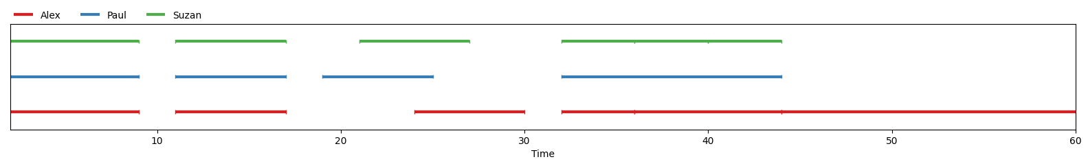
The same image can also be displayed with matplotlib by using :

from pygamma_agreement import show_continuum
show_continuum(continuum, labelled=True)

Alignments, Unitary Alignments

A unitary alignment is a tuple of units, each belonging to a unique annotator. For a given continuum containing annotations from n different annotators, the tuple will have to be of length n. It represents a “match” (or the hypothesis of an agreement) between units of different annotators. A unitary alignment can contain empty units, which are “fake” (and null) annotations inserted to represent the absence of corresponding annotation for one or more annotators.

An alignment is a set of unitary alignments that constitute a partition of a continuum. This means that

• each and every unit of each annotator from the partitioned continuum can be found in the alignment

• each unit can be found once and only once

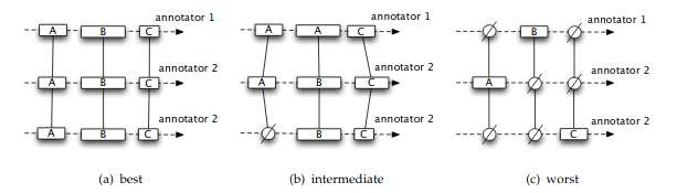
Visual representations of unitary alignments taken from [mathet2015] , with varying disorders.

For both alignments and unitary alignments, it is possible to compute a corresponding disorder. This possible via the compute_disorder method, which takes a dissimilarity as an argument. This (roughly) corresponds to the disagreement between annotators for a given alignment or unitary alignment.

In practice, you shouldn’t have to build both unitary alignments and alignments yourself, as they are automatically constructed by a continuum instance’s get_best_alignment method.

Best Alignments

For a given continuum, the alignment with the lowest possible disorder. This alignment is found using a combination of 3 steps:

• the computation of the disorder for all potential unitary alignments

• a simple heuristic explained in [mathet2015]’s section 5.1.1 to eliminate a big part of those potential unitary alignments based on their disorder

• the usage of multiple optimization problem formulated as Mixed-Integer Programming (MIP)

The function that implements these 3 steps is, by far, the most compute-intensive in the whole pygamma-agreement library. The best alignment’s disorder is used to compute the The Gamma (γ) agreement .

Disorders

The disorder for either an alignment or a unitary alignment corresponds to the disagreement between its constituting units.

• the disorder between two units is directly computed using a dissimilarity.

• the disorder between units of a unitary alignment is an average of the disorder of each of its unit couples

• the disorder of an alignment is the mean of its constituting unitary alignments’s disorders

What should be remembered is that a dissimilarity is needed to compute the disorder of either an alignment or a unitary alignment, and that its “raw” value alone isn’t of much use but it is needed to compute the γ-agreement.

Dissimilarities

A dissimilarity is a function that “tells to what degree two units should be considered as different, taking into account such features as their positions, their annotations, or a combination of the two.” [mathet2015]. A dissimilarity has the following mathematical properties:

• it is positive (\(dissim (u,v) > 0\)))

• it is symmetric ( \(dissim(u,v) = dissim(v,u)\) )

• \(dissim(x,x) = 0\)

Although dissimilarities do look a lot like distances (in the mathematical sense), they don’t necessarily are distances. Hence, they don’t necessarily honor the triangular inequality property.

If one of the units in the dissimilarity is the empty unit, its value is \(\Delta_{\emptyset}\). This value is constant, and can be set as a parameter of a dissimilarity object before it is used to compute an alignment’s disorder.

Right now, there are three types of dissimilarities available :

• The positionnal sporadric dissimilarity (we will call it simply Positionnal dissimilarity)

• The categorical dissimilarity

• The combined dissimilarity

Note

Although you will have to instantiate dissimilarities objects when using pygamma-agreement, you’ll never have to use them in any way other than just by passing it as an argument as shown beforehand.

Positional Dissimilarity

A positional dissimilarity is used to measure the positional or temporal disagreement between two annotated units \(u\) and \(v\).

[mathet2015] introduces the positional sporadic dissimilarity as the reference positional dissimilarity for the gamma-agreement. Its formula is :

\[d_{pos}(u,v) = \left( \frac{\lvert start(u) - start(v) \rvert + \lvert end(u) - end(v) \rvert} {(duration(u) + duration(v))} \right)^2 \cdot \Delta_{\emptyset}\]

Here’s how to instanciate a PositionnalSporadicDissimilarity object :

from pygamma_agreement import PositionalDissimilarity
dissim_pos = PositionalSporadicDissimilarity(delta_empty=1.0)

and that’s it. You can also use dissim_pos.d(unit1, unit2) to obtain directly the value of the dissimilarity between two units. It is however very unlikely that one would need to use it, as this value is only needed in the very low end of the gamma computation algorithm.

Categorical Dissimilarity

A categorical dissimilarity is used to measure the categorical disagreement between two annotated units \(u\) and \(v\).

\[d_{cat}(u,v) = dist_{cat}(cat(u), cat(v)) \cdot \Delta_{\emptyset}\]

In our case, the function \(dist_{cat}\) is computed using a simple lookup in a categorical distance matrix D. Let’s suppose we have \(K\) categories, this matrix will be of shape (K,K).

Here is an example of a distance matrix for 3 categories:

>>> D
array([[0. , 0.5, 1. ],
       [0.5, 0. , 1. ],
       [1. , 1. , 0. ]])

To comply with the properties of a dissimilarity, the matrix has to be symmetrical, and has to have an empty diagonal. Moreover, its values have be between 0 and 1. By default, for two units with differing categories, \(d_{cat}(u,v) = 1\), and thus the corresponding matrix is:

>>> D_default
array([[0., 1., 1. ],
       [1., 0., 1. ],
       [1., 1., 0. ]])

here’s how to instanciate a categorical dissimilarity:

D = array([[ 0.,   0.5,    1. ],
           [0.5,    0.,  0.75 ],
           [ 1.,  0.75,    0. ]])

from pygamma_agreement import PrecomputedCategoricalDissimilarity
from sortedcontainers import SortedSet

categories = SortedSet(('Noun', 'Verb', 'Adj'))
dissim_cat = PrecomputedCategoricalDissimilarity(categories,
                                            matrix=D,
                                            delta_empty=1.0)

Warning

It’s important to note that the index of each category in the categorical dissimilarity matrix is its index in alphabetical order. In this example, the considered dissimilarity will be:

• \(dist_{cat}('Adj', 'Noun') = 0.5\)

• \(dist_{cat}('Adj', 'Verb') = 1.0\)

• \(dist_{cat}('Noun', 'Verb') = 0.75\)

You can also use the default categorical dissimilarity, the AbsoluteCategoricalDissimilarity; there are also other available categorical dissimilarities, such as the LevenshteinCategoricalDissimilarity which is based on the levenshtein distance.

Combined Dissimilarity

The combined categorical dissimilarity uses a linear combination of the two previous categorical and positional dissimilarities. The two coefficients used to weight the importance of each dissimilarity are \(\alpha\) and \(\beta\) :

\[d_{combi}^{\alpha,\beta}(u,v) = \alpha . d_{pos}(u,v) + \beta . d_{cat}(u,v)\]

This is the dissimilarity recommended by [mathet2015] for computing gamma.

It takes the same parameters as the two other dissimilarities, plus \(\alpha\) and \(\beta\) :

from pygamma_agreement import CombinedCategoricalDissimilarity, LevenshteinCategoricalDissimilarity

categories = ['Noun', 'Verb', 'Adj']
dissim = CombinedCategoricalDissimilarity(alpha=3,
                                          beta=1,
                                          delta_empty=1.0,
                                          pos_dissim=PositionalSporadicDissimilarity()
                                          cat_dissim=LevenshteinCategoricalDissimilarity(categories))

The Gamma (γ) agreement

The γ-agreement is a chance-adjusted measure of the agreement between annotators. To be computed, it requires

• a continuum , containing the annotators’s annotated units.

• a dissimilarity, to evaluate the disorder between the hypothesized alignments of the annotated units.

Using these two components, we can compute the best alignment and its disorder. Let’s call this disorder \(\delta_{best}\).

Without getting into its details, our package implements a method of sampling random annotations from a continuum. Using these \(N\) sampled continuum, we can also compute a best alignment and its subsequent disorder. Let’s call these disorders \(\delta_{random}^i\), and the mean of these values \(\delta_{random} = \frac{\sum_i \delta_{random}^i}{N}\)

The gamma agreement’s formula is finally:

\[\gamma = 1 - \frac{\delta_{best}}{\delta_{random}}\]

Several points that should be clarified about that value:

• it is bounded by \(]-\infty,1]\) but for most “regular” situations it should be contained within \([0, 1]\)

• the higher and the closer it is to 1, the more similar the annotators’ annotations are.

the gamma value is computed from a Continuum object, using a given Dissimilarity object :

continuum = Continuum.from_csv('your/csv/file.csv')
dissim = CombinedCategoricalDissimilarity(delta_empty=1,
                                          alpha=3,
                                          beta=1)
gamma_results = continuum.compute_gamma(dissim,
                                        precision_level=0.02)

print(f"gamma value is: {gamma_results.gamma}")

Warning

The algorithm implemented by continuum.compute_gamma is very costly. An approximation of its computational complexity would be \(O(N \times (p_1 \times ... \times p_n))\) where \(p_i\) is the number of annotations for annotator \(i\), and \(N\) is the number of samples used when computing \(\delta_{random}\), which grows as the precision_level parameter gets closer to 0. If time of computation becomes too high, it is advised to lower the precision before anything else.

Gamma-cat (γ-cat) and Gamma-k (γ-k)

\(γ_{cat}\) is an alternate inter-annotator agreement measure based on γ, made to evaluate the task of categorizing pre-defined units. Just like γ, it is a chance-adjusted metric :

\[\gamma_{cat} = 1 - \frac{\delta_{best}^{cat}}{\delta_{random}^{cat}}\]

Where the disorder \(\delta_{cat}\) of a continuum is computed using the same best alignment used for the γ-agreement : this disorder is basically the average dissimilarity between pairs of non-empty units in every unitary alignment, weighted by the possitional agreement between the units.

The \(γ_{cat}\)-agreement can be obtained from the GammaResults object easily:

print(f"gamma-cat value is : {gamma_results.gamma_cat} ")

\(γ_{k}\) is another alternate agreement measure. It only differs from \(γ_{cat}\) by the fact that it only considers one defined category.

The \(γ_{k}\) value for a category alse can be obtained from the GammaResults object:

for category in continuum.categories:
    print(f"gamma-k of '{category}' is : {gamma_results.gamma_k(category)} ")

Further details about the measures and the algorithms used for computing them can be consulted in [mathet2015].

On a side-note, we would recomment combining gamma-cat with the alternate inter-annotator user agreement measure Soft-Gamma (new measure whose idea emerged during the developpement of pygamma-agreement). More information about soft-gamma is available in the dedicated section of this documentation.

[mathet2015] (1,2,3,4,5,6,7,8)

Yann Mathet et Al. The Unified and Holistic Method Gamma (γ) for Inter-Annotator Agreement Measure and Alignment (Yann Mathet, Antoine Widlöcher, Jean-Philippe Métivier)

[mathet2018]

Yann Mathet The Agreement Measure Gamma-Cat : a Complement to Gamma Focused on Categorization of a Continuum (Yann Mathet 2018)